4. Data & Evaluation Toolkit: Preparing and Analyzing the Data
Last Updated: 5/07/25

How to Use This Section:
Explore concepts, vocabulary, and approaches relating to preparing and analyzing data.
What is data preparation and analysis?
Before diving into the analysis step, datasets first need to be prepared. This process, referred to as data preparation or data cleaning, involves identifying and addressing inaccurate, irrelevant, duplicative, and incomplete data. It may also involve reformatting data in ways more convenient for analysis. Data is often messy and can be riddled with data entry errors such as typos, misspellings, and missing responses. This data preparation step is critical to make sure the analysis is based on data that is as accurate and complete as possible.
Once data is prepared, it is now ready for analysis. Data analysis involves processing prepared data to uncover trends, patterns, and other useful information. These analysis efforts aim to provide insights which can be used to address the project’s key question.
A number of different tools are commonly used for data preparation and analysis, including:
Excel, Google Sheets, Python, R, SAS, SPSS, and Stata. Check out the guides and resources from New York University, Princeton University, and University of California Irvine to learn more about each of these tools.
The remainder of this section introduces key vocabulary and concepts relating to data preparation and analysis. This discussion is geared towards those unfamiliar with this work or those who need a refresher – it will not teach all the technical information necessary to carry out full analysis efforts. For those interested in learning about specific data analysis techniques, check out
Coursera and Harvard University which both offer a range of free, online classes on this subject.
How is data prepared and why does it matter?
As a best practice, data preparation starts with duplicating and saving a complete copy of the original dataset. This ensures that the raw, unedited data is always available for reference as needed.
The following example dataset from a case management system will be used to review common data preparation steps. Please note that this example, with only 9 rows of data, is very simplified; data preparation will often involve hundreds to millions of data points.

To prepare data, look out for errors, inconsistencies, and missing or irrelevant data. Examples of steps to take to clean the above dataset include:
- Correcting Data Entry Errors: Case #6242 is listed with a 1022 intake date, a clear typo that can be changed to 2022. This is a reasonable assumption to make, because the because the case management system was not available until the 2000s (so the intake date would not be 1922). When it is unclear how to correct an apparent typo, do not change the data because the adjusted information may be incorrect.
Resolving Inconsistent Entries: Respondents manually type in the client’s city of residence, resulting in two cases (#1363 and #8335) with different spellings for the same location, “Brooklyn” and “Bkyln”. Decide on a standard way to list this city name and record it for both cases. - Addressing Missing Data: The client’s gender is unknown for cases #8335 and #2355. If possible, reach out to the data entry source to complete the missing data point. If this is not possible, decide on a standard way to mark missing gender values and adhere to that rule for all cases where client gender is not known.
- Reviewing Outliers: The client’s age is listed as 113 for case #6242, which is almost certainly a typo. If possible, go back to the source to confirm if this information is correct and adjust if necessary. If this is not possible, one approach would be to remove client age as a data point for case #6264 and treat this as missing data. In this example, the attorney was able to confirm the client’s correct age was 13, so 113 can be replaced with 13.
- Removing Irrelevant Data: The analysis will focus on cases with 2022 intake dates, so case #9234 and its entire row of data can be removed because the intake took place in 2019.
- Removing Duplicate Data: Case #7345 appears twice in the dataset, with the exact same information in all cells. Only one row per unique case is needed for the analysis, so one of the two rows for case #7345 can be removed.
Data preparation is critical because it ensures the analysis is as accurate as possible. If the above dataset is not properly cleaned, there are clear, negative impacts on the analysis as shown below:
- Failing to address data entry errors and inconsistencies can result in incorrect analysis. For example, if “Brooklyn” and “Bkyln” are left as is, this would appear as two distinct locations in a summary of total cases by city.
- Results can be skewed if outliers are not addressed. For example, if the client age of 113 is left in, the mean client age in the data set would be 53. If it is replaced with the correct value (13), the mean client age is 42.
- If irrelevant or duplicative data is not removed, incorrect analysis may result. For example, if the 2019 case is left in the dataset, this would inflate the total intake in 2022 by one.
While the exact steps needed to properly prepare data will vary depending on the source data, the examples above represent common approaches taken to produce a clean dataset. The following is an example of the dataset listed above, now prepared and ready for analysis:

How is data analyzed?
Data analysis refers to the processing of prepared data to uncover trends, patterns, and other useful information. There are four categories of analysis that aim to address slightly different questions: descriptive, diagnostic, predictive, and prescriptive. The following chart highlights the different aims of these types of analysis:

See the Harvard Business School's guide on data analysis for improved decision making for more information on these four types of data analysis.
The remainder of this section focuses on the common components of descriptive analysis, which plays a role in the simplest to the most complex data analysis undertakings. Advanced data analysis techniques are beyond the scope of this toolkit, which are typically needed in diagnostic, predictive, and prescriptive analyzes.
Descriptive analysis uses data to highlight trends and phenomena that are relevant to addressing the key question of the project. Descriptive analysis includes measures of:
- Frequency: Describes how often values occur within a dataset (e.g., totals, ratios).
- Central Tendency: Describes the central or most typical value of a particular data point (e.g., mean, median, mode).
- Dispersion: Describes the spread of the data from the center (e.g., range, standard deviation).
- Position: Describes where a value falls in the distribution of all values in the dataset (e.g., quartiles, percentiles).
These measures, in combination, shed light on different aspects and trends of a dataset. To demonstrate this, let’s return to the prepared (or cleaned) dataset from the previous section, which will now be used to demonstrate various descriptive statistic calculations:
| Case ID | Intake Date | Status | Client’s City of Residence | Client Age | Gender | Unique Client ID |
|---|---|---|---|---|---|---|
| 1363 | 3/21/2022 | Open | Brooklyn | 28 | Male | #12 |
| 6242 | 2/1/2022 | Closed | Manhattan | 13 | Female | #56 |
| 8335 | 8/11/2022 | Open | Brooklyn | 75 | Unknown | #74 |
| 7345 | 6/17/2022 | Closed | Queens | 28 | Female | #18 |
| 3992 | 5/21/2022 | Closed | Queens | 41 | Female | #92 |
| 2355 | 1/9/2022 | Open | Manhattan | 67 | Unknown | #77 |
| 4121 | 9/2/2022 | Open | Bronx | 43 | Male | #41 |
First, let’s calculate various descriptive statistics for client age, using the above dataset of 7 unique clients:
Name of Measure | Definition | Example Measure from the Dataset | Calculation |
|---|---|---|---|
Total | A count of values | 4 clients are 40+ | Counted the number of clients with an age of 40 or above |
Ratio | A comparison of two or more values | 57% of clients are 40+ | Counted the number of clients with an age of 40 or above and divided by the total number of clients: 4 / 7 |
Mean | The average value | 42 years | Added all client ages and divided by the total number of clients: [13 + 28 + 28 + 41 + 43 + 67 + 75] / 7 |
Median | The center value | 41 years | Arranged all client ages from lowest to highest and located the middle number: 13, 28, 28, 41, 43, 67, 75 |
Mode | The most common value | 28 years | Reviewed the client ages to identify which age was the most frequently recurring |
Range | The difference between the maximum and minimum value | 62 years | Subtracted the maximum and minimum ages: 75 - 13 |
Standard Deviation | An indication of how spread out the data is relative to the mean | 22 years; each age deviates from the mean by 22 years, on average. | Coursera provides a free instruction video on calculating standard deviation.* |
Coursera Training on Standard Deviation
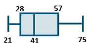
Data can also be summarized by quartiles, which involves sorting the data in numeric order and dividing it into four equal parts. For the above dataset: 21 is the minimum value, 28 years is the 1st quartile, 41 years is median (2nd quartile), 57 is the 3rd quartile, and 75 is the maximum value. Quartiles are another helpful measure to showcase the spread of the data, and can be showcased with a box plot, as exemplified below:
These different measurements - frequency, central tendency, dispersion, and position – identity spread, outliers, common values, and potential relationships of data points. Descriptive analysis summaries often include measures across these four categories, to help showcase different aspects of the data.
Descriptive analysis can involve looking at one data point on its own (univariate analysis), as with the above example on client age. It can also reference a combination of two data points (bivariate analysis) or several data points (multivariate analysis). Using the example dataset from above, a simple example of bivariate descriptive analysis is the following table of clients by gender and county of residence:
| Female | Male | Unknown | Total |
|---|---|---|---|---|
Bronx | 0 | 1 | 0 | 1 |
Brooklyn | 0 | 1 | 1 | 2 |
Manhattan | 1 | 0 | 1 | 2 |
Queens | 2 | 0 | 0 | 2 |
Total | 3 | 2 | 2 | 7 |
Keep in mind that descriptive analysis measures (median, mean, etc.) are not always feasible, depending on the data point’s level of measurement (nominal, ordinal, interval, or ratio).
For example, take a sample of 10 people, of which 3 are female and 7 are male. Gender uses a nominal scale. Nominal scales are categories, which have no numeric significance and have no meaningful order. For this sample, it would be impossible to calculate the “mean” gender. However, it would be possible to calculate the mode (the most common value), which would be male (since 7 of the 10 people are male).
The chart below depicts this relationship between level of measurement and analysis options in greater detail, highlighting whether it is possible to calculate a given metric for each measurement level:
| Total | Mode | Median | Mean | Standard Deviation | |
|---|---|---|---|---|---|
| Definition of Measure | A count of values | The most common value | The center value | The average value | An indication of how spread out the data is relative to the mean |
Nominal | Yes | Yes | No | No | No |
Ordinal | Yes | Yes | Yes | Sometimes | No |
Interval | Yes | Yes | Yes | Yes | Yes |
Ratio | Yes | Yes | Yes | Yes | Yes |
Moving forward in the data analysis project, the next section reviews strategies to present on and learn from the analysis.